Drawing with Constraints

Introduction

CAD constraints are geometric and dimensional rules that define how sketch or assembly entities relate to one another. They control degrees of freedom (for example, parallel, perpendicular, tangent, coincident, distance, or angle), so edits preserve design intent instead of introducing unintended shape changes. This is the foundation of parametric modeling: behavior is driven by explicit relationships, not fixed manually drawn geometry. This section only addresses sketch constraints.

In graphical CAD systems, sketching is usually a two-step workflow: first draw approximate geometry, then add dimensions and constraints so a global solver can infer exact positions. That model works well for interactive drawing, but it also encourages tightly coupled constraint networks that can become difficult to predict and maintain as a design evolves. It is also typically strongest for lines and circular arcs, with more limited and less robust behavior for ellipses, splines, and other higher-order curves.

In build123d, the primary workflow is different. Geometry is defined precisely at creation time using coordinates, parameters, and explicit geometric relationships in code. Instead of building a large interdependent constraint graph and asking a global solver to resolve it, you express intent directly: mirror about a plane, construct tangent features, derive points and frames from existing topology, and compose operations deterministically.

This does not eliminate constrained construction; it scopes it. build123d provides targeted geometric local solvers for common high-value problems, including objects such as BlendCurve, ConstrainedLines, ConstrainedArcs, and Triangle. It also provides a growing family of constructors whose extent can be determined by other geometry, including PolarLine, CenterArc, EllipticalCenterArc, EllipticalStartArc, JernArc, ParabolicCenterArc, and HyperbolicCenterArc. Together with operations such as make_hull, mirror, and offset, these tools solve specific constraint patterns while keeping model behavior explicit, deterministic, and readable in code.

The result is a practical hybrid approach: precise programmatic modeling by default, with specialized constrained constructors when they provide clear leverage. For most production parts, this yields robust, maintainable sketches without the overhead and fragility of a general-purpose sketch solver.

Constraint Types

build123d supports several practical forms of constrained construction. Rather than relying on a single global sketch solver, it provides targeted tools that enforce specific geometric relationships directly and predictably.

Analytical Constraints

Triangle

Constructs a triangle from any three parameters (side lengths and/or interior angles) and solves for the others. Angle naming follows standard convention: side a is opposite angle A, side b is opposite angle B, and side c is opposite angle C.

Continuity Constraints

BlendCurve

Creates a smooth Bézier transition between two existing edges.

In this context, continuity describes how smoothly the new blend joins the input edges at each endpoint:

• C0 (positional continuity): endpoints meet, but direction may kink.

• C1 (tangent continuity): endpoints and tangent directions match, giving a visually smooth join with no corner.

• C2 (curvature continuity): endpoints, tangents, and curvature trend match, reducing curvature jumps and producing a smoother fairing.

BlendCurve builds a Bézier curve that satisfies these endpoint constraints:

• cubic Bézier for C1 blending (position + first derivative),

• quintic Bézier for C2 blending (position + first and second derivatives).

The derivatives are sampled from the two source edges at the selected connection points, then converted into Bézier control points that enforce the requested continuity. Optional tangent scaling factors let you tune how strongly the blend departs from each source edge, which adjusts perceived tension and transition shape without changing the endpoint constraints.

Geometric Relationship Constraints

@ and % operators

Use @ (position-at) and % (tangent-at) to construct geometry relative to existing geometry. Typical uses include starting a new edge at an exact point on another edge, or aligning a new edge direction to a sampled tangent.

mirror

Enforces symmetry by reflecting geometry about a plane, producing mirrored entities with exact geometric correspondence to the source.

Extent / Termination Constraints

PolarLine, CenterArc, EllipticalCenterArc, EllipticalStartArc, JernArc, ParabolicCenterArc, and HyperbolicCenterArc

Construct curves from natural geometric parameters, then let another object determine where the result ends.

In these constructors, the size argument can often be either:

• a numeric angular or linear extent, or

• a limiting object such as a Shape, Axis, Location, Plane, or point-like object.

When a limit object is provided, the constructor creates the candidate geometry from the supplied start conditions, trims it at the first valid intersection with the limit, and returns the shortest valid result from the start. If no valid intersection exists, a ValueError is raised.

This pattern is especially useful when design intent is "go in this direction until you meet that object", because it removes helper construction lines and separate trim calls while keeping the relationship local to the constructor call.

Offset / Equidistance Constraints

offset

Creates geometry at a constant normal distance from a source edge or wire.

This enforces an equidistance relationship commonly used for wall thickness, clearances, toolpaths, and parallel profile construction. Join behavior (for example at corners) can be controlled to match the design intent.

Tangency Constraints

ConstrainedArcs and ConstrainedLines

Provide local constrained solving for 2D line-and-circle constructions. These APIs solve common geometric construction problems from explicit numeric and geometric constraints relative to existing curves.

Supported constraint patterns include:

• circle with specified radius,

• line at a specified angle to another line,

• tangency of a line or circle to a reference curve,

• line or circle passing through a point,

• circle center constrained to a point or to lie on a curve.

For example, you can construct a circle with a given radius whose center lies on a specified line and which is tangent to another circle. This style of targeted solving covers high-value sketch workflows while keeping branch selection explicit and deterministic in code.

Multiple Solutions and Qualification

Tangency construction is typically multi-solution. A single problem statement can produce several valid geometric branches depending on where the solution lies relative to the reference entities.

For example, a circle of fixed radius tangent to two secant circles can produce up to eight valid solutions as shown below. This is expected behavior, not an error.

To reduce ambiguity, tangency constraints support qualification of relative position:

• Tangency.ENCLOSING: the solution must enclose the argument.

• Tangency.ENCLOSED: the solution must be enclosed by the argument.

• Tangency.OUTSIDE: the solution and argument must be external to each other.

• Tangency.UNQUALIFIED: no positional filtering; all valid branches are returned.

These qualifiers are intuitive for circles (inside/outside). For general oriented curves, interior is defined as the left-hand side of the curve with respect to its orientation.

Even with qualification, more than one solution may remain. In that case, use a selector to choose deterministic outputs.

Selecting results

In Algebra mode, select from returned edges after construction:

arcs = ConstrainedArcs(..., sagitta=Sagitta.BOTH)
chosen = arcs.edges().sort_by(Edge.length)[0]

In Builder mode, prefer the constructor selector argument so only desired branches are added to the active context:

with BuildLine():
   ConstrainedArcs(
         ...,
         selector=lambda edges: edges.sort_by_distance((0, 0))[0],
   )

This combination of qualification + selection gives robust, explicit control over tangency branch choice.

Practical Examples

The following examples show how each constraint type is used in production-style sketching. Each example is intentionally small, with construction geometry kept visible in code so the relationship logic is explicit and reusable.

Analytical Constraints

build123d includes a built-in Triangle object that has an internal solver such that one can specify any three parameters of a triangle and solve for the others. For example:

>>> isosceles = Triangle(a=30, b=30, C=60)
>>> isosceles.c
29.999999999999996
>>> isosceles.A
60.00000000000001
>>> isosceles.B
60.00000000000001
>>> isosceles.vertex_A
Vertex(-1.7763568394002505e-15, 17.32050807568877, 0.0)

In this example, side lengths a and b with included angle C are provided. The object then computes the remaining side, angles, and vertices. This is useful when a design intent is naturally expressed as triangle dimensions instead of explicit coordinates.

One can easily use external solvers, say the symbolic solver sympy, within your build123d code as follows:

from math import sin, cos, tan, radians
from build123d import *
from ocp_vscode import *
import sympy

# This problem uses the sympy symbolic math solver

# Define the symbols for the unknowns
# - the center of the radius 30 arc (x30, y30)
# - the center of the radius 66 arc (x66, y66)
# - end of the 8° line (l8x, l8y)
# - the point with the radius 30 and 66 arc meet i30_66
# - the start of the horizontal line lh
y30, x66, xl8, yl8 = sympy.symbols("y30 x66 xl8 yl8")
x30 = 77 - 55 / 2
y66 = 66 + 32

# There are 4 unknowns so we need 4 equations
equations = [
   (x66 - x30) ** 2 + (y66 - y30) ** 2 - (66 + 30) ** 2,  # distance between centers
   xl8 - (x30 + 30 * sin(radians(8))),  # 8 degree slope
   yl8 - (y30 + 30 * cos(radians(8))),  # 8 degree slope
   (yl8 - 50) / (55 / 2 - xl8) - tan(radians(8)),  # 8 degree slope
]
# There are two solutions but we want the 2nd one
solution = {k: float(v) for k,v in sympy.solve(equations, dict=True)[1].items()}

# Create the critical points
c30 = Vector(x30, solution[y30])
c66 = Vector(solution[x66], y66)
l8 = Vector(solution[xl8], solution[yl8])

...

This pattern is useful when the governing relationships are algebraic but awkward to construct directly with primitives. Solve unknown parameters first, then feed the solved values into standard build123d geometry construction.

Continuity Constraints

One may want to join two curves with a third curve such that the connector satisfies a given continuity where they meet as shown here where a semi-circle (on the left) is joined to a spline (on the right).

m1 = CenterArc((-2, 0.6), 1, -10, 200).reversed()
m2 = Spline((0.4, -0.6), (1, -1.6), (2, 0))
connector = BlendCurve(m1, m2, tangent_scalars=(2, 1), continuity=ContinuityLevel.C2)
comb = Curve(Wire([m1, connector, m2]).curvature_comb(200))

The key call is BlendCurve(..., continuity=ContinuityLevel.C2). C2 continuity matches endpoint curvature trend in addition to position and tangent, which reduces visible fairness breaks at joins. tangent_scalars controls how strongly the connector departs from each source curve.

curvature_comb is used here as a diagnostic. The normal "comb" lines represent local curvature magnitude; smoother transitions produce gradual comb variation rather than abrupt spikes.

Geometric Relationship Constraints

Coincident

with BuildLine() as coincident_ex:
   l1 = Line((0, 0), (1, 2))
   l2 = Line(l1 @ 1, l1 @ 1 + (1, 0))

The second line starts at l1 @ 1 (the end of l1), creating an exact coincident relationship without a separate constraint object.

Tangent

with BuildLine() as tangent_ex:
   l1 = Line((0, 0), (1, 1))
   l2 = JernArc(start=l1 @ 1, tangent=l1 % 1, radius=1, arc_size=70)

The arc starts at the line endpoint and uses l1 % 1 as its initial tangent direction. This is a direct tangent construction: continuity is encoded in the creation call.

Perpendicular

with BuildLine() as perpendicular_ex:
   l1 = CenterArc((0, 0), 1.5, 0, 45)
   l2 = PolarLine(
      start=l1 @ 1, length=1, direction=l1.tangent_at(1).rotate(Axis.Z, -90)
   )

The direction vector is built from l1.tangent_at(1) rotated by 90 degrees, giving an explicit perpendicular relationship relative to curve orientation.

Extent / Termination Constraints

with BuildLine() as intersect_ex:
   c1 = EllipticalCenterArc((0, 0), 1.2, 1.8, 0, arc_size=120, mode=Mode.PRIVATE)
   l1 = PolarLine(start=(-0.2, 0.1), length=c1, angle=10)
   l2 = PolarLine(start=(-0.2, 0.1), length=c1, angle=70)
   l3 = add(c1.trim(l1 @ 1, l2 @ 1))

PolarLine creates each line from a start point and direction, then limits it by intersection with the ellipse. This is often cleaner than creating long helper lines and manually trimming afterward, and the same pattern applies to a wide range of arcs and conics.

The same extent-by-object pattern works with several curved constructors:

• CenterArc

• EllipticalCenterArc

• EllipticalStartArc

• JernArc

• ParabolicCenterArc

• HyperbolicCenterArc

For example, a parabola or hyperbola can be grown from a start condition and terminated by a line or axis in the same way:

p1 = ParabolicCenterArc((0, 0), 0.5, 0, arc_size=Line((0, 1), (5, 1)))
h1 = HyperbolicCenterArc((0, 0), 2, 1, 0, arc_size=Axis((0, 1), (1, 0)))

This is particularly useful when sketches are not symmetric and multiple local constructions must terminate against different surrounding geometry.

Offset / Equidistance Constraints

inside = FilletPolyline((1.5, 0), (1.5, 1), (-1.5, 1), (-1.5, 0), radius=0.2)
perimeter = offset(inside, amount=0.2, side=Side.RIGHT)

offset preserves the source profile shape while enforcing constant wall thickness. This is a common pattern for clearances, shells, and manufacturing margins.

Tangency Constraints

Both ConstrainedArcs and ConstrainedLines return a Curve containing one or more Edge objects.

These constructors solve tangent/contact problems from mixed numeric and geometric inputs. Because tangency is often ambiguous, multiple valid branches are expected.

Multiple solutions

Constraint systems often yield multiple valid results. The selector callback is the main tool for choosing the subset to keep.

# Keep all solutions
ConstrainedArcs(..., selector=lambda arcs: arcs)

# Keep first
ConstrainedArcs(..., selector=lambda arcs: arcs[0])

# Keep shortest
ConstrainedArcs(..., selector=lambda arcs: arcs.sort_by(Edge.length)[0])

In Builder mode, omitting selector can add all solutions to context, which is often not what you want for production sketches.

Tangency qualifiers

Tangency qualifiers come from OCCT and are exposed as Tangency:

• Tangency.UNQUALIFIED: no side preference (OCCT Unqualified).

• Tangency.OUTSIDE: tangent on the exterior side of the target (OCCT Outside).

• Tangency.ENCLOSING: solution encloses/includes the target (OCCT Enclosing).

• Tangency.ENCLOSED: solution is enclosed/included by the target (OCCT Enclosed).

These semantics are most visible for curve-vs-curve constraints (for example circle to circle, line to circle). In many practical cases, UNQUALIFIED is a good default followed by filtering via selector.

with BuildLine() as egg_plant:
   # Construction Geometry
   c1 = CenterArc((-2, 0), 0.75, 80, 240, mode=Mode.PRIVATE)
   c2 = CenterArc((2, 0), 1, 220, 250, mode=Mode.PRIVATE)

   # egg_plant perimeter
   l1 = ConstrainedArcs((c2, Tangency.OUTSIDE), (c1, Tangency.OUTSIDE), radius=6)
   l2 = ConstrainedArcs(
      (c2, Tangency.ENCLOSING),
      (c1, Tangency.ENCLOSING),
      radius=8,
      selector=lambda a: a.sort_by(Axis.Y)[-1],
   )
   l3 = add(c1.trim(l1 @ 1, l2 @ 1))
   l4 = add(c2.trim(l1 @ 0, l2 @ 0))

In the "egg-plant" example, Tangency.OUTSIDE and Tangency.ENCLOSING reduce the candidate branches to the intended outer profile. The selector on l2 then resolves the remaining ambiguity deterministically by choosing the highest branch in Y.

OCCT defines exterior/interior using orientation:

• Circle: exterior is on the right side when traversing by its orientation (interior/material is on the left side).

• Line/open curve: interior is the left side with respect to traversal direction, exterior is the opposite side.

Because of this, changing an input edge direction can change which branches satisfy OUTSIDE/ENCLOSING/ENCLOSED.

If qualifier behavior appears inverted, inspect input edge orientation first.

ConstrainedArcs

Overview

ConstrainedArcs supports several signature families for planar circular arcs:

1. Two tangency/contact objects + fixed radius

2. Two tangency/contact objects + center constrained on a locus

3. Three tangency/contact objects

4. One tangency/contact object + fixed center

5. One tangency/contact object + fixed radius + center constrained on a locus

sagitta selects short/long/both arc branches:

• Sagitta.SHORT

• Sagitta.LONG

• Sagitta.BOTH

In practice, use qualifiers and sagitta to reduce branch count, then finalize with selector for deterministic output.

Signature A: Two constraints + radius

ConstrainedArcs(
    tangency_one,
    tangency_two,
    radius=...,
    sagitta=Sagitta.SHORT,
    selector=lambda arcs: arcs,
)

Use when radius is known and arc must satisfy two contact/tangency conditions.

Signature B: Two constraints + center_on

ConstrainedArcs(
    tangency_one,
    tangency_two,
    center_on=Axis(...),  # or Edge
    sagitta=Sagitta.SHORT,
    selector=lambda arcs: arcs,
)

Use when center must lie on a specific line/curve rather than radius being fixed.

Signature C: Three constraints

ConstrainedArcs(
    tangency_one,
    tangency_two,
    tangency_three,
    sagitta=Sagitta.BOTH,
    selector=lambda arcs: arcs,
)

Use for "arc tangent/contact to three entities". This can produce several branches; always consider using selector.

Signature D: One constraint + fixed center

ConstrainedArcs(
    tangency_one,
    center=(x, y),
    selector=lambda arcs: arcs[0],
)

Useful for "center-known" constructions.

Signature E: One constraint + radius + center_on

ConstrainedArcs(
    tangency_one,
    radius=...,
    center_on=some_edge,
    selector=lambda arcs: arcs,
)

Useful for guided-center constructions with fixed radius.

Allowed constraint objects

For arc constraints, accepted objects include:

• Edge

• Axis

• Vertex / VectorLike point

• optional qualifier wrapper: (object, Tangency.XXX)

ConstrainedLines

Overview

ConstrainedLines supports these signature families:

1. Tangent/contact to two objects

2. Tangent/contact to one object and passing through a fixed point

3. Tangent/contact to one object with fixed orientation (angle or direction)

Signature A: Two constraints

ConstrainedLines(
    tangency_one,
    tangency_two,
    selector=lambda lines: lines,
)

Signature B: One constraint + through point

ConstrainedLines(
    tangency_one,
    (x, y),  # through point
    selector=lambda lines: lines,
)

Signature C: One constraint + fixed orientation

ConstrainedLines(
    tangency_one,
    Axis.Y,
    angle=30,              # OR direction=(dx, dy)
    selector=lambda lines: lines,
)

Exactly one of angle or direction should be provided.

For all signatures, qualifiers can be attached to tangency inputs when side selection must be controlled.

Builder vs Algebra mode

Algebra mode

Use direct assignment and post-selection:

arcs = ConstrainedArcs(..., sagitta=Sagitta.BOTH)
chosen = arcs.edges().sort_by(Edge.length)[0]

Builder mode

Prefer selecting inside the call to avoid adding unwanted candidates to context:

with BuildLine() as bl:
    ConstrainedArcs(
        ...,
        sagitta=Sagitta.BOTH,
        selector=lambda arcs: arcs.sort_by(Edge.length)[0],
    )

Selection recipes

# Nearest to point
selector=lambda edges: edges.sort_by_distance((0, 0))[0]

# Longest
selector=lambda edges: edges.sort_by(Edge.length)[-1]

# Right most
selector=lambda edges: edges.sort_by(Axis.X)[-1]

# Keep two branches
selector=lambda edges: edges[:2]

Prefer geometric selection criteria (distance, axis ordering, length) over positional indexing when upstream geometry may change.

Complex Drawing Example

This example pulls many of the techniques described above into a single example where the following full constrained, complex sketch is converted into build123d code.

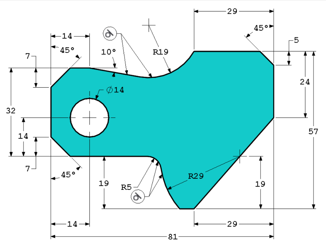
When working with a drawing such as this one, the ImageFace functionality of the ocp-vscode viewer is very handy as it allows the image to be used as a visual guide when creating the sketch.

Within the following code the following conventions are used:

• construction geometry is labeled with a c_...

• arcs are labeled with a a<radius>

• lines and polylines are labeled with a l...

The code starts immediately above the origin (arbitrarily set to the origin of the circle) where a straight line 10° off the x-axis originates. The code then walks around the diagram clockwise creating the perimeter of the object.

image = ImageFace(
   "complex_sketch.png",
   scale=29 / 264,
   origin_pixels=(297, 390),
   location=Location((0, 0, -0.1)),
)

with BuildSketch() as sketch:
   with BuildLine() as perimeter:
      c_l1 = PolarLine((0, 32 - 14), 50, -10, mode=Mode.PRIVATE)
      a19 = ConstrainedArcs(c_l1, (-14 + 81 - 29, -14 - 19 + 57), radius=19)
      l2 = Polyline(a19 @ 1, a19 @ 1 + (29 - 5, 0), a19 @ 1 + (29, -5), (-14 + 81, 0))
      l3 = Line(l2 @ 1, (-14 + 81 - 29, (-14 - 19)))
      c_l4 = Line((-14, -14), (-14 + 81, -14), mode=Mode.PRIVATE)
      c_a29_arc_center = l3.intersect(c_l4)[0]
      c_a29 = CenterArc(c_a29_arc_center, 29, 180, 50, mode=Mode.PRIVATE)
      l5 = PolarLine(l3 @ 1, length=c_a29, direction=(-1, 0))
      a5 = ConstrainedArcs(
            c_a29, c_l4, radius=5, selector=lambda a: a.sort_by(Axis.X)[0]
      )
      a29 = add(c_a29.trim(l5 @ 1, a5 @ 0))
      l6 = Polyline(
            a5 @ 1,
            (-14 + 7, -14),
            (-14, -14 + 7),
            (-14, -14 + 32 - 7),
            (-14 + 7, -14 + 32),
            (0, -14 + 32),
            a19 @ 0,
      )
   make_face()
   a14 = Circle(14 / 2, mode=Mode.SUBTRACT)

Implementation notes:

1. Build in traversal order around the perimeter. This keeps references local and makes later edits easier because each segment depends on nearby geometry.

2. Keep helper entities private (mode=Mode.PRIVATE) so only final profile edges contribute to the resulting face.

3. Use named construction geometry (c_...) for intersections and arc centers; this improves readability and debugability.

4. Use constrained constructors only where they add value (for example ConstrainedArcs), and use direct primitives elsewhere.

5. Create a Face (make_face then center-hole subtraction) only after the perimeter is fully defined.

Troubleshooting

• Too many results: add qualifiers and a stricter selector.

• No results: relax qualifier (start with UNQUALIFIED) and verify geometry is coplanar.

• Unstable branch selection: avoid index-only selection when topology changes; prefer geometric sorting.

• Builder mode unexpectedly adds many edges: provide selector explicitly in the constructor call.